Breathing New Life into Old Maps by Making Them 3D with Rayshader
- Jacob Benzaquen

- Mar 22, 2021
- 5 min read
Last year, while browsing reddit, I first encountered Rayshader, a package in R created by Tyler Morgan-Wall, and fell in love. I started out by making 3D maps of Landsat satellite imagery, as well as different types of tiled, and line based heightmaps. More recently, I encountered a few recreations of old maps by other creators on Twitter, and had to lock myself down for a few days to try it for myself.
Preface
Before we begin, I would like to reiterate that there may be better ways to do what I am doing, and I am still very new to writing code. I have had a lot of help with different aspects from different creators, and pieces of the code are copied and pasted form Tyler Morgan-Walls Github, and this blog.
I will also be using Rstudio, so all of my instructions will be referencing that. We will also need QGIS for georeferencing.
In this post I will be working on an old Geologic map of Mt. Myaki-Jima in Japan.
Required Packages
For this tutorial we will need three different packages. Raster, Rayshader, and Elevatr.
To download these in Rstudio:
Click on Tools--Install Packages--Search the name of the package, and hit install.
Data
The first thing we need to obtain is the map itself. You can find this from multiple sources, and old map Catalogs. My favorites are David Rumsey's Map Catalog, USGS Topo View, USGS Map View, and where we will get this one, Japan Geological Survey.
One important thing to note about the maps, is that they need to be georeferenced, i.e. it needs a coordinate system. You can usually tell if it is by the file type. geotiffs are almost always referenced, while regular .tif, .jpg, and .png are not.
On the Japan Geological Survey, they have every type, but the full map, is only in.jpg format, so we will have to georeference in QGIS.
Download the Myaki-Jima Map jpg Here
Georeferencing in QGIS
Note: This is not mandatory if you downloaded a geotiff file. Skip to Here if you did
Open up QGIS, and click on New Empty Project
On the top tool bar click on Raster--Georeferencer. This will open up the new window.
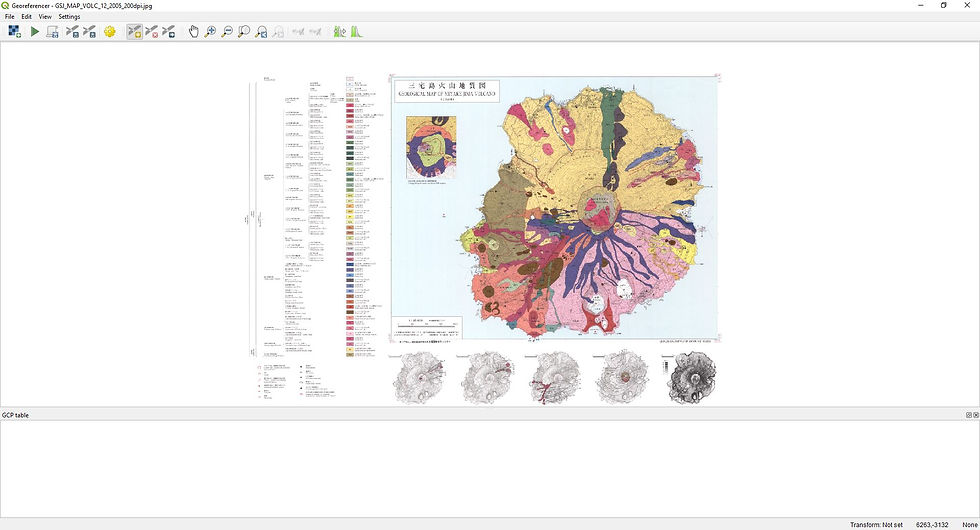
Click on File--Open Raster and open up the Map
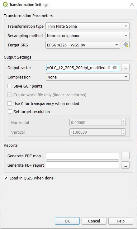
Click on the yellow settings button and copy these settings. You can pretty much use these universally for all of these maps. Make sure to hit the 3 dots next to output raster and save it in a good location.
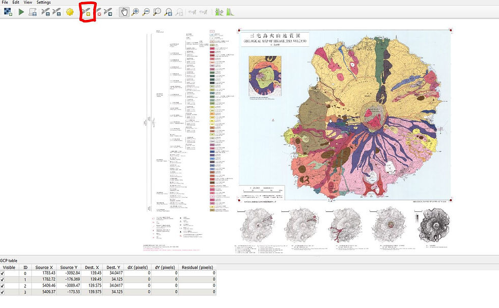
Then Click on the add point tool, zoom in, and add a coordinate point on each of the four corners. They will usually be labeled on these maps. If you are unfamiliar with degree coordinates, you may need to put them into this calculator.
Note: I entered them in in the order of: Bottom Left--Top Left--Bottom Right--Top Right because that will be helpful later.
Hit the green play button, and it will save the new geotiff file in your desired location.
Note: If you open it and see a lot of black around the edges, you can crop that out and resave in QGIS by hitting Raster--Extraction--Clip Raster By Extent, and draw a bounding box around the map. You will have to resave this new file.
Don't Close the georeferencer, as we can copy these coordinates later.
Elevation Data
You can always go out and search for the elevation data yourself, but Jhollist created a handy package to do that for us, elevatr.
Open RStudio and create a new Rscript.
Load in your packages
library(raster)
library(rayshader)
library(elevatr)
Set working directory to folder location
setwd("D:/Maps/Old Map")Import your Map File
topo_map <- topo_map <- raster::brick("myakyijima.tif")
topo_map <- raster::stack(topo_map)
To get the elevation file, we will use the elevatr package. The z value is the resolution of the height map. I usually use a 9 or a 10. Larger the map, the smaller the number.
elevation <- get_elev_raster(topo_map, z = 10)
plot(elevation)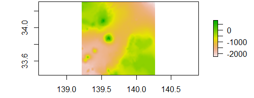
Fix Elevation Data
We could leave the elevation as is, but it would stretch out to the edges of the map, including over the words, so let's crop it out by the maps coordinate lines. Remember to keep the same order of the coordinates as above: Bottom Left, Top Left, Bottom Right, Top right.
#crop elevation to map
elevation <- raster::crop(elevation, extent(topo_map))

#Bring down elevation past map lines
base_raster <- elevation * 0 + 450

# Crop to Map Lines
x <- c(139.450, 139.450, 139.575, 139.575)
y <- c(34.042, 34.125, 34.042, 34.125)
xy <- cbind(x,y)
S <- SpatialPoints(xy, proj4string = CRS("+proj=longlat +ellps=clrk66 +datum=NAD27 +no_defs "))

S <- spTransform(S, crs(topo_map))

interior_elevation <- raster::crop(elevation, extent(S))

elevation <- merge(interior_elevation, base_raster)
Now we have to lay the map image on top of the elevation data. To do this, Tyler requires that the map needs to be split into a 3 channel RGB Layer. Most of this is a copy and paste from his blog.
names(topo_map) <- c("r", "g", "b")
topo_r <- rayshader::raster_to_matrix(topo_map$r)
topo_g <- rayshader::raster_to_matrix(topo_map$g)
topo_b <- rayshader::raster_to_matrix(topo_map$b)
topo_rgb_array <- array(0, dim = c(nrow(topo_r), ncol(topo_r), 3))

topo_rgb_array[,,1] <- topo_r/255
topo_rgb_array[,,2] <- topo_g/255
topo_rgb_array[,,3] <- topo_b/255

# Transpose map
topo_rgb_array <- aperm(topo_rgb_array, c(2,1,3))
Time To Rayshade!
We need to convert to a matrix first to make this work using raster_to_matrix(). The ray_shade() function calculates a shadow map from the elevation matrix, the ambient_shade() calculates the Ambient Occlusion Shadow Map. I can't touch on this as much as it goes over my head.
elev_mat <- raster_to_matrix(elevation)
ray_shadow <- ray_shade(elev_mat, sunaltitude = 40, zscale = 30, multicore = TRUE)
ambient_shadow <- ambient_shade(elev_mat, zscale = 30)
Create the "flat" 3D Map
elev_mat %>%
  sphere_shade(texture = "bw") %>%
  add_overlay(topo_rgb_array) %>%
  add_shadow(ray_shadow, max_darken = 0.7) %>%
  add_shadow(ambient_shadow, 0.25) %>%
  plot_map()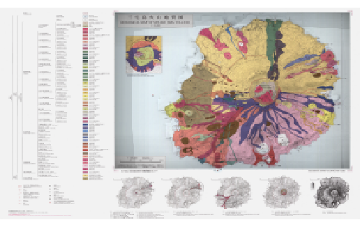
Make it 3D
We only need a few lines of code to make this 3D. This will open up a new rgl window with the 3d map, although it will be ugly and have no shadows. From here you can play around with this with your mouse.
plot_3d(topo_rgb_array,elev_mat, zscale = 20, windowsize = c(1800,2400),
        phi = 40, theta = 135, zoom = 0.9,
        background = "grey30", shadowcolor = "grey5",
        soliddepth = -50, shadowdepth = -100)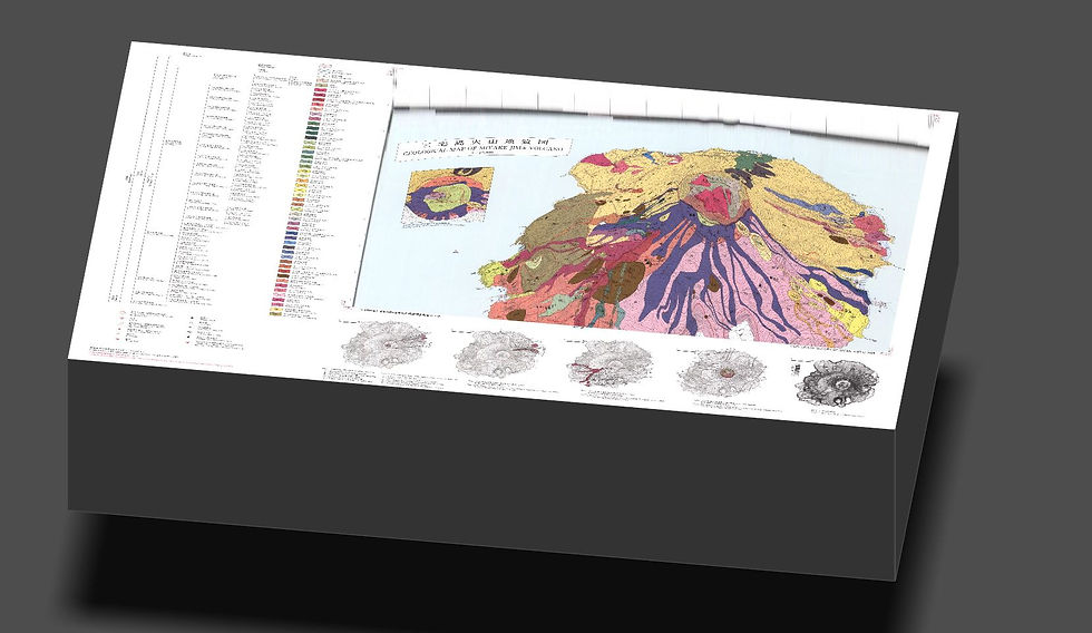
Now we want to make this higher quality with raytraced shadows. You first need to pass render_camera to get it to the correct angle, before passing render_highquality. Feel free to play around with any of the numbers, and reference Tyler's Github for more you can add.
Note: These are two angles I have found work well for these. Uncomment the one you want to do.
Note2: This will not work if you played around in the rgl window at all. Close and re run the plot_3d before running these if you did. One cool thing you can do is add a cool light source by downloading from here, and adding in environment_light('filename') into render_highquality.
#render_camera(theta = 0, phi = 89, zoom = 0.7, fov = 0)
#render_camera(theta = -0, phi = 60, zoom = 0.12, fov = 150)
render_highquality('myakijima.png', lightintensity = 500, samples = 400, width = 7200, height = 4800, lightdirection = 290)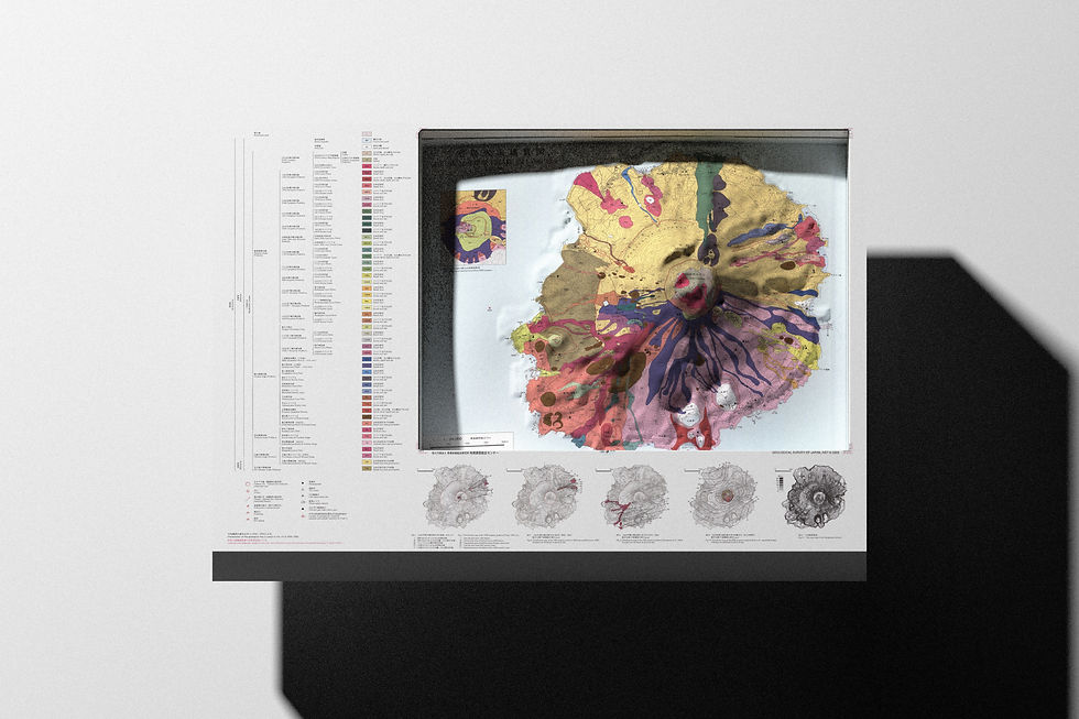
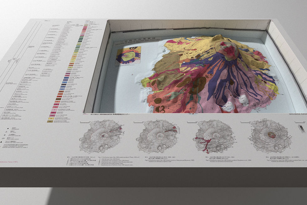

You can also create a movie by passing this code, although I have not figured out how to make that the highquality image, so any help there would be great!
render_movie(filename = "myakijima.mp4", type = "orbit",
             phi = 40,theta = 0,frames = 1440, fps = 60)
Please make sure to comment any that you have done, or any suggestions.
Follow me on Twitter!
References:
Schramm (2020, Oct. 9). @mpschramm: Rayshading maps. Retrieved from https://michaelpaulschramm.com/posts/2020-10-08-rayshading_maps/
Replicating:
code can be found on my GitHub
https://github.com/BigBallerBenzie/OldMap
Corrections:
For any corrections, please comment, or reach out to me directly.
Citations:
To cite this source, please use this format:
Benzaquen (2021, Mar. 22). @mpschramm: Breathing New Life into Old Maps by Making Them 3D with Rayshader. Retrieved from https://jacobbenzaquen53.wixsite.com/website/blog
.png)
Comments